In R, error metrics are essential tools used in machine learning, statistics, and data analysis to evaluate the performance of models. These metrics quantify the difference between predicted values and actual values. Below are some of the common error metrics used in regression and classification problems:

1.  Mean Absolute Error (MAE)

• Description: MAE is the average of the absolute differences between predicted and actual

Formula:

where yi is the actual value and yi^yi^ is the predicted value.

R Code

# Function to calculate MAE

mae <- function(actual, predicted) {

    mean(abs(actual – predicted))

}

# Example usage

actual <- c(3, -0.5, 2, 7)

predicted <- c(2.5, 0.0, 2, 8)

mae(actual, predicted)

Interpretation:

• The smaller the MAE, the better the model’s predictions are on

‍

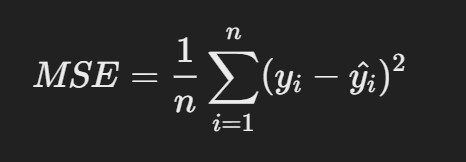
2.  Mean Squared Error (MSE)

• Description: MSE measures the average squared differences between predicted and actual values. It gives higher weight to larger errors than MAE.

R Code

# Function to calculate MSE

mse <- function(actual, predicted) {

    mean((actual – predicted)^2)

}

# Example usage

mse(actual, predicted)

Interpretation:

• Smaller MSE values indicate better model Larger errors have a higher impact due to the squaring of differences.

‍

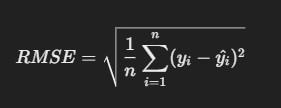
3.  Root Mean Squared Error (RMSE)

• Description: RMSE is the square root of MSE, making it more interpretable as it’s in the same units as the actual values.

Formula

R Code:

# Function to calculate RMSE

rmse <- function(actual, predicted) {

sqrt(mean((actual – predicted)^2))

}

# Example usage

rmse(actual, predicted)

Interpretation:

• RMSE is useful when large errors are more significant than small errors, and lower RMSE values represent a better fit of the model.

4.  R-squared (R²)

• Description: R² measures the proportion of the variance in the dependent variable that is predictable from the independent variables.

Formula

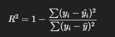
where yˉ is the mean of the actual values..

R Code

where yˉ is the mean of the actual values..

# Function to calculate R²

rsq <- function(actual, predicted) {

1 – sum((actual – predicted)^2) / sum((actual – mean(actual))^2)

}

# Example usage

rsq(actual, predicted)

‍

Interpretation:

• R² values closer to 1 indicate that the model explains a large proportion of the variance, while values closer to 0 indicate poor explanatory power.

‍

5.  Adjusted R-squared

• Description: Adjusted R² accounts for the number of predictors in the model, adjusting R² by penalizing the addition of unnecessary predictors.

Formula:

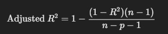
where n is the number of data points and pp is the number of predictors.

R Code:

# Example using a linear model

model <- lm(mpg ~ wt + hp, data = mtcars) summary(model)$adj.r.squared

Interpretation:

Adjusted R² is better for comparing models with different numbers of predictors, as it accounts for model complexity.

‍

6.  Mean Absolute Percentage Error (MAPE)

• Description: MAPE measures the accuracy of a model as a percentage, by averaging the absolute percentage errors.

Formula:

R Code

# Function to calculate MAPE

mape <- function(actual, predicted) { mean(abs((actual – predicted) / actual)) * 100

}

# Example usage

mape(actual, predicted)

Interpretation:

• A lower MAPE value indicates a more accurate model, especially useful for models with varied scales.

‍

7.  Logarithmic Loss (LogLoss)

• Description: LogLoss is commonly used in classification It measures the

uncertainty of predictions by penalizing wrong classifications with a higher penalty when confidence is high.

Formula:

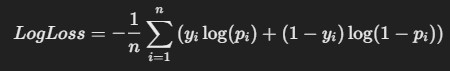
where yi is the actual class (0 or 1), and pi is the predicted probability for class 1.

R Code

where yi is the actual class (0 or 1), and pi is the predicted probability for class 1.

# Function to calculate LogLoss

logloss <- function(actual, predicted_prob) {

-mean(actual * log(predicted_prob) + (1 – actual) * log(1 -predicted_prob))

}

# Example usage

actual <- c(1, 0, 1, 1, 0)

predicted_prob <- c(0.9, 0.1, 0.8, 0.7, 0.2)

logloss(actual, predicted_prob)

Interpretation:

• Lower LogLoss indicates a better-performing classifier, especially when handling probabilistic

8.  Confusion Matrix & Related Metrics (for Classification Problems)

Description: A confusion matrix provides a summary of the classification performance by showing the counts of true positives, false positives, true negatives, and false negatives.

R Code:

# Example using the caret package

library(caret)

actual <- factor(c(1, 0, 1, 1, 0))

predicted <- factor(c(1, 0, 1, 0, 0))

confusionMatrix(predicted, actual)

‍