Data Warehousing 101: Star Schema vs Snowflake Schema

If you have ever written a SQL query that joins six tables to answer a simple business question, you have felt the pain of poorly designed data models. Data warehousing exists to solve this problem — organizing data so that analytics and reporting are fast, intuitive, and reliable.

At the heart of data warehouse design is a choice between two schema patterns: star schema and snowflake schema. Understanding when and why to use each is fundamental knowledge for any data engineer, analyst, or BI developer.

What is a Data Warehouse?

A data warehouse is a centralized repository designed specifically for analytical queries and reporting. Unlike your transactional database (which handles day-to-day operations), a data warehouse is optimized for reading and aggregating large volumes of historical data.

Key characteristics:

• Subject-oriented — Organized around business subjects (sales, customers, inventory) rather than application processes
• Integrated — Consolidates data from multiple source systems into a consistent format
• Time-variant — Maintains historical data to enable trend analysis over time
• Non-volatile — Data is loaded in bulk and rarely updated or deleted once written

OLTP vs OLAP

Before diving into schema design, it is crucial to understand the distinction between the two systems:

Feature	OLTP (Transactional)	OLAP (Analytical)
Purpose	Day-to-day operations	Reporting and analysis
Query type	INSERT, UPDATE, DELETE (single rows)	SELECT with aggregations (millions of rows)
Data model	Highly normalized (3NF)	Denormalized (star/snowflake)
Users	Application users, software	Analysts, business users, dashboards
Data freshness	Real-time current state	Periodic loads (hourly/daily) or near-real-time
Optimization	Write performance	Read performance
Example	MySQL/PostgreSQL for your application	BigQuery/Redshift/Snowflake for analytics
Schema design	ER diagrams, normalized tables	Dimensional modeling (facts + dimensions)

Your application database (OLTP) is not designed for analytics. Running complex aggregation queries on it will slow down your production application. That is why data is extracted, transformed, and loaded (ETL) into a separate data warehouse (OLAP) that is optimized for those queries.

Dimensional Modeling: Facts and Dimensions

Data warehouse schemas are built on dimensional modeling, a technique introduced by Ralph Kimball. The idea is simple but powerful:

Fact Tables

A fact table stores the measurable events of your business — transactions, clicks, orders, payments. Each row represents one event.

Fact tables contain:

• Foreign keys linking to dimension tables
• Measures (numeric values you want to aggregate) — revenue, quantity, discount, cost

Example: A fact_sales table with columns like date_key, product_key, store_key, customer_key, quantity_sold, revenue, discount_amount.

Dimension Tables

A dimension table stores the descriptive context around your facts — the who, what, where, when.

Example dimensions:

• dim_product — product name, category, subcategory, brand, price tier
• dim_customer — customer name, segment, city, state, registration date
• dim_store — store name, location, region, format (online/offline)
• dim_date — date, day of week, month, quarter, year, fiscal period, is_holiday

Dimension tables are typically wide (many columns) but short (thousands to millions of rows), while fact tables are narrow (few columns) but tall (millions to billions of rows).

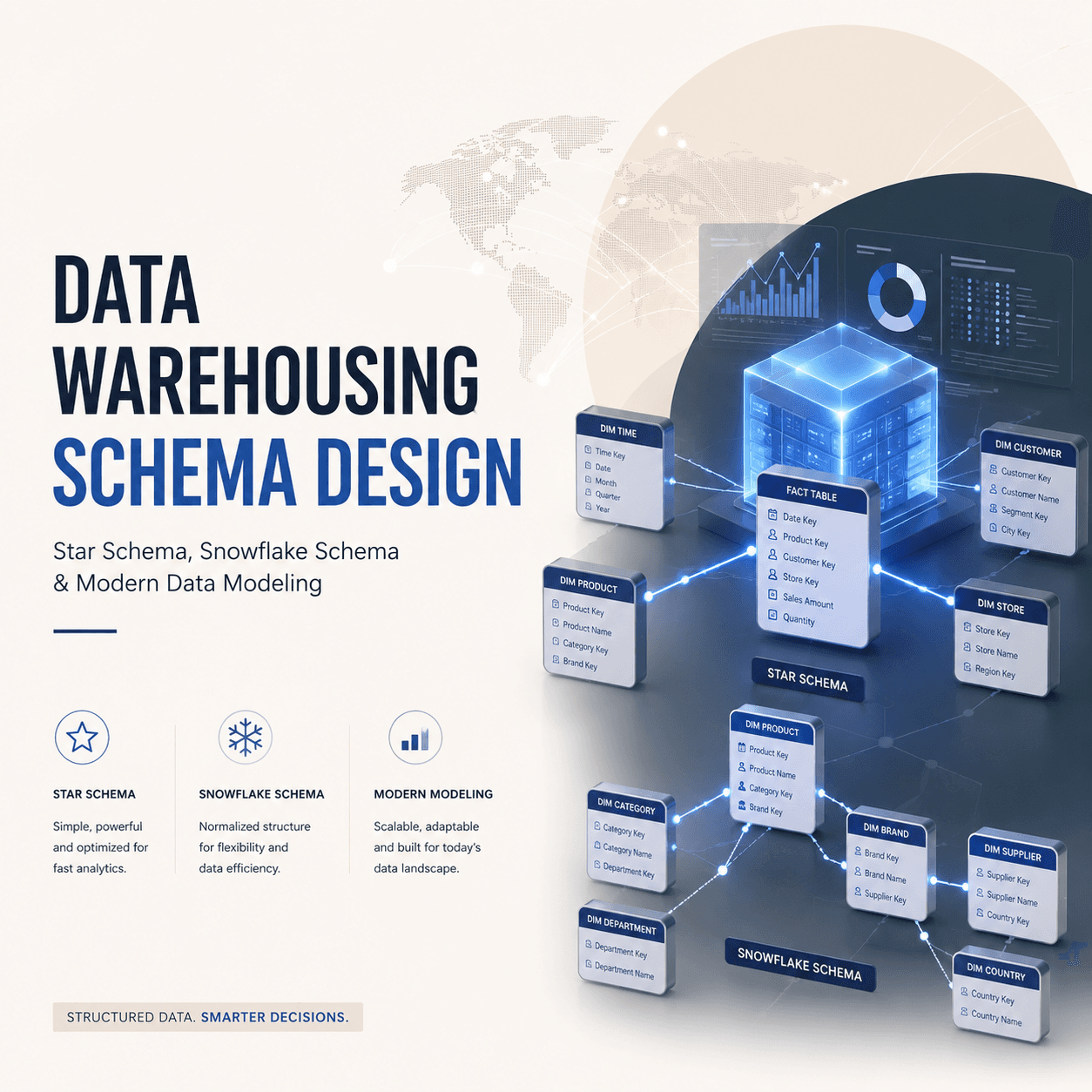
Star Schema Explained

The star schema is the simplest and most widely used data warehouse schema. It gets its name from its shape — a central fact table connected directly to dimension tables, forming a star pattern.

Structure

The fact table sits at the center. Each dimension table connects directly to the fact table via a foreign key relationship. Dimension tables are denormalized — all descriptive attributes are stored in a single flat table.

For an e-commerce data warehouse:

• Center: fact_orders (order_key, date_key, product_key, customer_key, store_key, quantity, revenue, discount)
• Points of the star:
  • dim_date (date_key, full_date, day_name, month, quarter, year)
  • dim_product (product_key, product_name, category, subcategory, brand)
  • dim_customer (customer_key, name, email, city, state, segment)
  • dim_store (store_key, store_name, city, state, region, format)

Star Schema Query Example

-- Total revenue by product category and quarter
SELECT
    d.quarter,
    p.category,
    SUM(f.revenue) AS total_revenue,
    COUNT(DISTINCT f.order_key) AS total_orders
FROM fact_orders f
JOIN dim_date d ON f.date_key = d.date_key
JOIN dim_product p ON f.product_key = p.product_key
WHERE d.year = 2025
GROUP BY d.quarter, p.category
ORDER BY d.quarter, total_revenue DESC;

Notice how clean this query is — one fact table, two simple joins, and you have your answer. This is the power of star schema.

Advantages of Star Schema

• Simple queries — Fewer joins, intuitive structure, easy for analysts to understand
• Fast performance — Denormalized dimensions mean fewer joins at query time
• BI tool friendly — Tools like Tableau, Power BI, and Looker work naturally with star schemas
• Easy to maintain — Adding a new dimension is straightforward

Snowflake Schema Explained

The snowflake schema is a variation of the star schema where dimension tables are normalized into multiple related tables. Instead of storing all product attributes in one dim_product table, you split them into separate tables.

Structure

Using the same e-commerce example:

• Center: fact_orders (same as star schema)
• Normalized dimensions:
  • dim_product (product_key, product_name, subcategory_key, brand_key)
  • dim_subcategory (subcategory_key, subcategory_name, category_key)
  • dim_category (category_key, category_name)
  • dim_brand (brand_key, brand_name, country_of_origin)

The dim_product table no longer contains category or brand names directly — it references them through foreign keys to normalized lookup tables.

Snowflake Schema Query Example

-- Total revenue by product category and quarter (snowflake version)
SELECT
    d.quarter,
    cat.category_name,
    SUM(f.revenue) AS total_revenue,
    COUNT(DISTINCT f.order_key) AS total_orders
FROM fact_orders f
JOIN dim_date d ON f.date_key = d.date_key
JOIN dim_product p ON f.product_key = p.product_key
JOIN dim_subcategory sub ON p.subcategory_key = sub.subcategory_key
JOIN dim_category cat ON sub.category_key = cat.category_key
WHERE d.year = 2025
GROUP BY d.quarter, cat.category_name
ORDER BY d.quarter, total_revenue DESC;

Notice the extra joins — you must traverse through dim_product to dim_subcategory to dim_category to get the category name.

Star Schema vs Snowflake Schema

Feature	Star Schema	Snowflake Schema
Dimension structure	Denormalized (flat)	Normalized (multiple tables)
Number of joins	Fewer (simpler queries)	More (complex queries)
Query performance	Faster (fewer joins)	Slower (more joins)
Storage efficiency	More redundancy	Less redundancy
Ease of understanding	Very intuitive	More complex to navigate
ETL complexity	Simpler to load	More complex transformations
BI tool compatibility	Excellent	Good (but more configuration)
Data integrity	Lower (denormalized)	Higher (normalized)
Maintenance	Easier	Harder (more tables to manage)
Best for	Analytics, dashboards, BI	Large-scale warehouses with strict storage constraints

When to Use Star Schema

• Your primary users are business analysts and BI tools
• Query performance is the top priority
• Your dimension tables are not excessively large
• You want simplicity in both querying and ETL

When to Use Snowflake Schema

• Storage cost is a major concern and dimension data has significant redundancy
• You need strict data integrity with no duplication
• Your ETL processes already normalize data naturally
• Dimension tables are very large with many shared attributes

In practice, star schema is the dominant choice for most modern data warehouses. The storage savings from snowflake schema are negligible with today's columnar storage engines (BigQuery, Redshift, Snowflake), and the query simplicity of star schema is a massive productivity gain.

Real-World Example: E-Commerce Data Warehouse

Let us design a simple data warehouse for an Indian e-commerce company (think Flipkart or Meesho):

Fact Table: fact_orders

CREATE TABLE fact_orders (
    order_key       BIGINT PRIMARY KEY,
    date_key        INT REFERENCES dim_date(date_key),
    product_key     INT REFERENCES dim_product(product_key),
    customer_key    INT REFERENCES dim_customer(customer_key),
    seller_key      INT REFERENCES dim_seller(seller_key),
    payment_key     INT REFERENCES dim_payment_method(payment_key),
    quantity        INT,
    gross_amount    DECIMAL(12,2),
    discount        DECIMAL(12,2),
    net_revenue     DECIMAL(12,2),
    shipping_cost   DECIMAL(10,2),
    is_returned     BOOLEAN
);

Sample Dimension: dim_customer

CREATE TABLE dim_customer (
    customer_key    INT PRIMARY KEY,
    customer_id     VARCHAR(20),    -- natural key from source system
    full_name       VARCHAR(100),
    email           VARCHAR(100),
    phone           VARCHAR(15),
    city            VARCHAR(50),
    state           VARCHAR(50),
    pin_code        VARCHAR(6),
    tier_city       VARCHAR(10),    -- Tier 1, Tier 2, Tier 3
    segment         VARCHAR(20),    -- Premium, Regular, New
    registration_date DATE,
    effective_from  DATE,           -- SCD Type 2 fields
    effective_to    DATE,
    is_current      BOOLEAN
);

Slowly Changing Dimensions (SCD)

Real-world dimension data changes over time. A customer moves to a new city. A product gets reclassified into a different category. How do you handle these changes?

SCD Type 1: Overwrite

Simply overwrite the old value with the new value. No history is maintained.

• Customer moves from Mumbai to Pune? Update the city column to "Pune".
• Pros: Simple, no extra storage
• Cons: You lose historical context. Past orders will appear as if they were from Pune.

SCD Type 2: Add New Row

Create a new row for the changed record, with version tracking fields (effective_from, effective_to, is_current).

• Customer moves from Mumbai to Pune? The old row gets effective_to = 2025-05-04, is_current = false. A new row is inserted with city = Pune, effective_from = 2025-05-05, is_current = true.
• Pros: Full history preserved. Past orders correctly link to the Mumbai version.
• Cons: Table grows larger. Queries need to filter on is_current = true for current state.

SCD Type 3: Add New Column

Add a column to store the previous value alongside the current value.

• Add previous_city and current_city columns.
• Pros: Simple to query both current and previous state
• Cons: Only tracks one level of history. Does not scale for multiple changes.

SCD Type 2 is the most commonly used approach in production data warehouses because it preserves complete history while maintaining accurate relationships with fact data.

Modern Data Warehouse Tools

The data warehouse landscape has shifted dramatically toward cloud-native, serverless platforms:

• Google BigQuery — Serverless, pay-per-query, excellent for organizations already on GCP. Supports nested/repeated fields (semi-structured data). Widely used by Indian startups.
• Amazon Redshift — Columnar storage, integrates tightly with the AWS ecosystem. Offers Redshift Serverless for variable workloads.
• Snowflake — Multi-cloud (AWS, Azure, GCP), separates compute from storage (scale independently). Known for its data sharing and marketplace features.
• Databricks Lakehouse — Combines data lake and data warehouse on Delta Lake. Strong for teams that need both ML and BI on the same platform.
• Apache Hive / Presto — Open-source options for organizations running on-premise Hadoop clusters. Still used in many Indian enterprises.

For most new projects in India, BigQuery and Snowflake are the most popular choices due to their ease of setup and managed infrastructure.

Best Practices for Schema Design

• Start with business questions — Design your schema to answer the queries your business actually needs, not to mirror your source system structure
• Prefer star schema — Unless you have a strong, specific reason for snowflake schema, star is almost always the better choice for analytics
• Use surrogate keys — Generate integer primary keys for dimension tables instead of using natural keys from source systems. This insulates your warehouse from source system changes.
• Build a robust dim_date — Pre-populate a date dimension with every date for 10+ years, including fiscal periods, holidays (Indian holidays are critical for retail analytics), and flags like is_weekend
• Implement SCD Type 2 for critical dimensions — At minimum, track history for customer, product, and employee dimensions
• Avoid wide fact tables — Keep fact tables narrow with only foreign keys and measures. If you need descriptive attributes in query results, join to dimension tables.
• Document your grain — Clearly define what one row in your fact table represents (one order line item? one transaction? one daily aggregate?). This is the most important design decision.
• Test with real queries — Before finalizing your schema, write the top 20 business queries your team needs and verify they can be expressed cleanly against your design

Data warehouse schema design is one of those skills where fundamentals matter more than tools. Platforms will change — BigQuery might be replaced by something new in five years — but the principles of dimensional modeling have remained relevant for three decades. Master the concepts, and the tools become interchangeable.