Meritshot Tutorials
- Home
- »
- Space and Time in Python
Python Tutorial
-
Understanding Variables in PythonUnderstanding Variables in Python
-
Types Of Operators in PythonTypes Of Operators in Python
-
How to create string ?How to create string ?
-
Data Structure in PythonData Structure in Python
-
What is a Function in PythonWhat is a Function in Python
-
Parameters and Arguments in PythonParameters and Arguments in Python
-
What is a Lambda FunctionWhat is a Lambda Function
-
What is a Regular Expression?What is a Regular Expression?
-
Introduction to Loops in PythonIntroduction to Loops in Python
-
If-else Statements in PythonIf-else Statements in Python
-
Break Statement in PythonBreak Statement in Python
-
OOPS in PythonOOPS in Python
-
Space and Time in PythonSpace and Time in Python
-
Data Type in PythonData Type in Python
Time Complexity and Big O Notation
An analogy to a real-life issue:
Suppose we have an issue which is :
This morning I wanted to eat some pizza; So, I asked my brother to get me some from Dominos, which is 3 km away.
He got me the pizza, and I was happy only to realize it was too little for 29 friends who came to my house for a surprise visit!
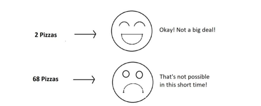
My brother can get 2 pizzas for me on his bike, but pizza for 29 friends is too huge of an input for him, which he cannot handle.
2 Pizza —-> Okay, it is possible*68 Pizza—– > Not quite possible*
What is Time Complexity?
Time Complexity is the study of the efficiency of algorithms. It tells us how much time is taken by an algorithm to process a given input. Let’s understand this concept with the help of an example:
Consider two developers Shubham(S) and Rohan(R), who created an algorithm to sort ‘n’ numbers independently. When I made the program run for some input size n, the following results aka time taken by both of them were recorded:
- 10 elemnets —> 90ms(S) —> 122ms(R)
- 70 elements —> 110 ms(S) —> 124ms(R)
- 110 elements —> 180ms(S) —> 131ms(R)
- 1000 elements —> 2s(S) > 800ms(R)
We can see that at first, Shubham’s algorithm worked well with smaller inputs; however, as we increase the number of elements, Rohan’s algorithm performs much better.
Who’s algorithm is better? What do you think ?
Time Complexity: Sending GTA 5 to a friend:
Imagine you have a friend who lives 5 km away from you. You want to send him a game. Since the final exams are over and you want him to get this 60 GB file worth of game from you. How will you send it to him
in the shortest time possible?
Note that both of you are using JIO 4G with a 1 Gb/day data limit.
The best way would be to send him the game by delivering it to his house. Copy the game to a hard disk and make it reach him physically.
Would you do the same for sending some small-sized game like MineSweeper which is in KBS of size? Of Course no, because you can now easily send it via the Internet.
As the file size grows, the time taken to send the game online increases linearly – O(n) while the time taken by sending it physically remains constant. O(n0) or O(1).
Calculating Order in terms of Input Size:
In order to calculate the order(time complexity), the most impactful term containing n is taken into account (Here n refers to Size of input). And the rest of the smaller terms are ignored.
Let us assume the following formula for the algorithms in terms of input size n:

Here, we ignored the smaller terms in algo 1 and carried the most impactful term, which was the square of the input size. Hence the time complexity became n^2. The second algorithm followed just a constant time complexity.
Note that these are the formulas for the time taken by their program.
What is a Big O?
Putting it simply, big O stands for ‘order of’ in our industry, but this is pretty different from the mathematical definition of the big O. Big O in mathematics stands for all those complexities our program runs in. But in industry, we are asked the minimum of them. So this was a subtle difference.
Visualizing Big O:
If we were to plot O(1) and O(n) on a graph, they would look something like this:

So, this was the basics of time complexities. Let’s look into them in a bit more detail.
Asymptotic Notations: Big O, Big Omega and Big Theta
Asymptotic notation gives us an idea about how good a given algorithm is compared to some other algorithm.
Now let’s look at the mathematical definition of ‘order of.’ Primarily there are three types of widely used asymptotic notations.
- Big oh notation ( O )
- Big omega notation ( Ω )
- Big theta notation ( θ ) – Widely used one
Big oh notation ( O ):
Big oh notation is used to describe an asymptotic upper bound. Mathematically, if f(n) describes the running time of an algorithm; f(n) is O(g(n)) if and only if there exist positive constants c and n° such that:
0 ≤ f(n) ≤ c g(n) for all n ≥ n°.
Here, n is the input size, and g(n) is any complexity function, for, e.g. n, n2, etc. (It is used to give upper bound on a function) If a function is O(n), it is automatically O(n2) as well! Because it satisfies the equation given above.
Graphic example for Big oh ( O ):

Big Omega Notation ( Ω ):
- Just like O notation provides an asymptotic upper bound, Ω notation provides an asymptotic lower bound.
- Let f(n) define the running time of an algorithm; f(n) is said to be Ω (g(n)) if and only if there exist positive constants c and n° such that:
0 ≤ c g(n) ≤ f(n) for all n ≥ n°.
- It is used to give the lower bound on a function.
If a function is Ω (n2) it is automatically Ω (n) as well since it satisfies the above equation.

Big theta notation ( θ ):
- Let f(n) define the running time of an algorithm.
F(n) is said to be θ (g(n)) if f(n) is O (g(n)) and f(x) is Ω (g(n)) both.
Mathematically,

Merging both the equations, we get:
0 ≤ c2 g(n) ≤ f(n) ≤ c1 g(n) ∀ n ≥ no.
The equation simply means that there exist positive constants c1 and c2 such that f(n) is sandwiched between c2 g(n) and c1 g(n).
Graphic example of Big theta ( θ ):

Which one of these to use?
Big theta provides a better picture of a given algorithm’s run time, which is why most interviewers expect you to answer in terms of Big theta when they ask “order of” questions. And what you provide as the answer in Big theta, is already a Big oh and a Big omega. It is recommended for this reason.
Increasing order of common runtimes:
Below mentioned are some common runtimes which you will come across in your coding career.

So, this was all about the asymptotic notations. We’ll come across these a lot in future.
Best Case, Worst Case and Average Case Analysis of an Algorithm
Life can sometimes be lucky for us:
Exams getting canceled when you are not prepared, a surprise test when you are prepared, etc. → Best case Occasionally, we may be unlucky:
Questions you never prepared being asked in exams, or heavy rain during your sports period, etc. → Worst case
However, life remains balanced overall with a mixture of these lucky and unlucky times. → Expected case
Those were the analogies between the study of cases and our everyday lives. Our fortunes fluctuate from time to time, sometimes for the better and sometimes for the worse. Similarly, a program finds it best when it is effortless for it to function. And worse otherwise.
By considering a search algorithm used to perform a sorted array search, we will analyze this feature.
Analysis of a search algorithm:
Consider an array that is sorted in increasing order. 1
7
18
28
50
180
We have to search a given number in this array and report whether it’s present in the array or not. In this case, we have two algorithms, and we will be interested in analyzing their performance separately.
Algorithm 1 – Start from the first element until an element greater than or equal to the number to be searched is found.
Algorithm 2 – Check whether the first or the last element is equal to the number. If not, find the number between these two elements (center of the array); if the center element is greater than the number to be searched, repeat the process for the first half else, repeat for the second half until the number is found. And this way, keep dividing your search space, making it faster to search.
Analyzing Algorithm 1: (Linear Search)
- We might get lucky enough to find our element to be the first element of the array. Therefore, we only made one comparison which is obviously constant for any size of the array.
Best case complexity = O(1)
- If we are not that fortunate, the element we are searching for might be the last one. Therefore, our program made ‘n’ comparisons.
Worst-case complexity = O(n) For calculating the average case time, we sum the list of all the possible case’s runtime and divide it with the total number of cases. Here, we found it to be just O(n). (Sometimes, calculation of average-case time gets very complicated.)
Analyzing Algorithm 2: (Binary Search)
If we get really lucky, the first element will be the only element that gets compared. Hence, a constant time.
Best case complexity = O(1)
- If we get unlucky, we will have to keep dividing the array into halves until we get a single element. (that is, the array gets finished) Hence the time taken : n + n/2 +n/4 +…………………………………………………………………………. + 1 = logn with base 2
Worst-case complexity = O(log n)
What is log(n)?
Logn refers to how many times I need to divide n units until they can no longer be divided (into halves).
log8 = 3 ⇒ 8/2 + 4/2 + 2/2 → Can’t break anymore.
- log4 = 2 ⇒ 4/2 + 2/2 → Can’t break anymore. You can refer to the graph below, and you will find how slowly
- the time complexity (Y-axis) increases when we increase the input n (X-axis).

Space Complexity:
The amount of memory an algorithm needs to run to completion. Measured in: Bytes or bits. Factors:
Input size (n)
Data structures used
Auxiliary space (extra memory) Now,
Time is not the only thing we worry about while analyzing algorithms. Space is equally important. Creating an array of size n (size of the input) → O (n) Space
If a function calls itself recursively n times, its space complexity is O (n)
You might have wondered at some point why we can’t calculate complexity in seconds when dealing with time complexities.
*Here’s why:
Not everyone’s computer is equally powerful. So we avoid handling absolute time taken. We just measure the growth of time with an increase in the input size. Asymptotic analysis is the measure of how time (runtime) grows with input.
Trade-offs:
Time vs. space: Often, there’s a trade-off between time complexity and space complexity. For example, using more space can sometimes lead to faster algorithms.
Example: Storing a List of Numbers
Let’s say you have a list of n numbers. If you make a copy of this list, you’ll need more memory.
def make_copy(numbers):
copied_list = numbers.copy()
return copied_list
In this example:
- The original list takes up n units of space.
The copied list also takes up n units of space. * Space Complexity: O(n)
- This means that the memory needed grows linearly with the size of the input.
Common Space Complexities
- O(1): Constant space. The algorithm uses the same amount of memory regardless of input size.
- O(n): Linear space. Memory usage grows proportionally with input size.
O(n^2): Quadratic space. Memory usage grows with the square of the input size.
Balancing Time and Space Complexity
Sometimes, you might have to choose between using less time or using less space. For example, you could save time by storing extra data, but that might use more memory.
Example: Caching Results
If you calculate something multiple times, you might store the result to save time later. But storing it will use more space
cache = {}
def expensive_calculation(x): if x in cache:
return cache[x] else:
result = x * x # Imagine that this is a complex operation
cache[x] = result return result
Balancing Time and Space Complexity
Understanding space-time complexity helps you write efficient code. Remember:
- Time Complexity measures how the runtime changes with input size.
Space Complexity measures how memory usage changes with input size.


