Meritshot Tutorials
- Home
- »
- Confidence Interval in R
R Tutorial
-
R-OverviewR-Overview
-
R Basic SyntaxR Basic Syntax
-
R Data TypesR Data Types
-
R-Data StructuresR-Data Structures
-
R-VariablesR-Variables
-
R-OperatorsR-Operators
-
R-StringsR-Strings
-
R-FunctionR-Function
-
R-ParametersR-Parameters
-
Arguments in R programmingArguments in R programming
-
R String MethodsR String Methods
-
R-Regular ExpressionsR-Regular Expressions
-
Loops in R-programmingLoops in R-programming
-
R-CSV FILESR-CSV FILES
-
Statistics in-RStatistics in-R
-
Probability in RProbability in R
-
Confidence Interval in RConfidence Interval in R
-
Hypothesis Testing in RHypothesis Testing in R
-
Correlation and Covariance in RCorrelation and Covariance in R
-
Probability Plots and Diagnostics in RProbability Plots and Diagnostics in R
-
Error Matrices in RError Matrices in R
-
Curves in R-Programming LanguageCurves in R-Programming Language
Confidence Interval in R
What is Confidence Intervals ?
A confidence interval is a range of values that is likely to contain the true value of a population parameter with a certain degree of confidence. It is commonly used in statistics to estimate the unknown population parameter (such as the mean or the proportion) based on a sample of data.
For example, if you want to estimate the average height of all people in a certain country, you can
take a sample of people and calculate their average height. However, this sample average may not be exactly equal to the true population average. A confidence interval provides a range of values that is likely to contain the true population average with a certain level of confidence (such as 95% or 99%).
So, a Confidence Interval is an interval of numbers containing the most plausible values for our Population Parameter. A point estimate gives a single value for a parameter. However, a point
estimate is not perfect and usually there is some error in the estimate. Instead of giving just a point estimate of a parameter, it would be better to provide a range of values for the parameter. A plausible range of values for the population parameter is called a confidence interval.
So basically, we try to build the confidence interval around the point estimate. The probability that this procedure produces an interval that contains the actual true parameter value is known as the Confidence Level and is generally chosen to be 0.9, 0.95 or 0.99.
Confidence Intervals (for a population mean) take the form:
Point Estimate +/- Critical Value x Standard Error

Z-scores are appropriate confidence coefficients for a confidence interval of the mean when the population standard deviation (σ) is known.
The level of confidence determines the z critical value.
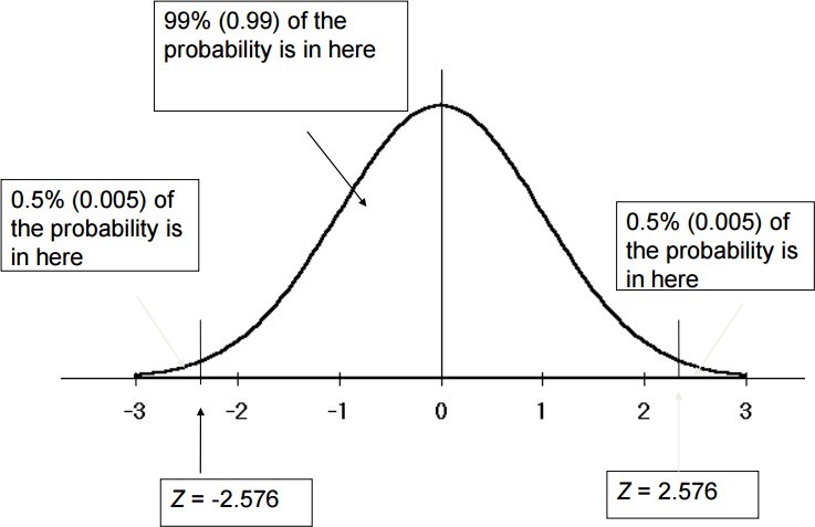
99% | 2.58 |
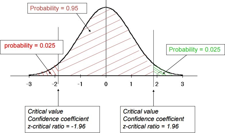
95% | 1.96 |
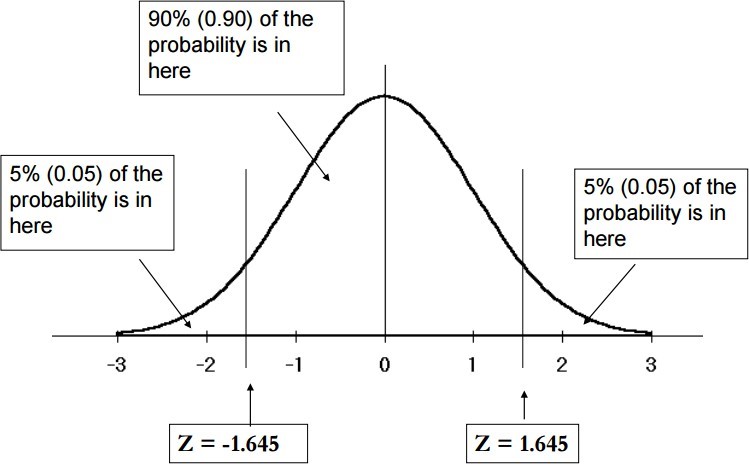
90% | 1.645 |
Confidence Coefficients for 99% Confidence Interval from standard normal distribution
Confidence Coefficients for 95% Confidence Interval from standard normal distribution
Confidence Coefficients for 90% Confidence Interval from standard normal distribution
However, most of the time when the population mean is being estimated from sample data the population variance is unknown and must also be estimated from sample data. The sample standard deviation (s) provides an estimate of the population standard deviation (σ).
Since n is large the unknown σ can be replaced by the sample value s.

The standard error represents the standard deviation associated with the estimate, and roughly 95% of the time the estimate will be within 2 standard errors of the parameter. If the interval spreads out 2 standard errors from the point estimate, we can be roughly 95% confident that we have captured the true parameter: point estimate ± 2 × SE. Similarly, we can construct 90% and 99% confidence interval using above z critical value.
Margin of error
In a confidence interval, z × SE is called the margin of error.
Conditions for confidence interval for Population mean
Some conditions need to be satisfied to use the above formula and to build the confidence interval. In fact, since this method is based on CLT it follows the same conditions for CLT.
- Independence: Sampled observations must be
- Random sample/random assignment
- If sampling without replacement, then needs to be n < 10% of
- Sample size/ skew: Either the population distribution is normal, or if the population distribution is skewed, the sample size is large (rule of thumb: n > 30)
If sample size is less than 30 then we use t-distribution.
Example:
A random sample of 225 1st year statistics tutorials was selected from the past 5 years and the
number of students absent from each one recorded. The results were x =11.6 and s=4.1 absences. Estimate the mean number of absences per tutorial over the past 5 years with 90% confidence.
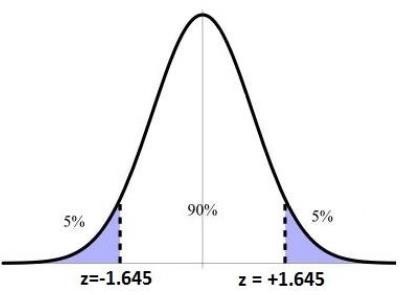
90% CI for μ is

How to Interpret the confidence intervals?
Suppose we took many samples and built a confidence interval from each sample using the above equation. Then about 90% of those intervals would contain the actual mean, µ. This is the correct interpretation of confidence interval.
So, we can say for the above example, 90% refers to the percentage of all possible intervals that contain μ i.e. to the estimation process rather than a particular interval.
It is incorrect to say that there is a probability of 0.90 that μ is between 11.15 and 12.05. In fact this probability is either 1 or 0 (μ either is or is not in the interval).
It is also incorrect to say that 90% of all tutorials had between 11.15 and 12.05 missing students.
Example 2:
A sample of 50 college students were asked how many exclusive relationships they’ve been in so far. The students in sample had an average of 3.2 exclusive relationship, with a standard deviation of
1.74. In addition, the sample distribution was slightly skewed to the right. Estimate the true average number of exclusive relationship based on this sample using 95% confidence interval.
So, n=50
¯x = 3.2
S= 1.74
We assume that the number of exclusive relationships one student in the sample has been in is independent of another. So, it is random and it is < 10% of all college student. On the other hand, n> 30 and not so skewed. So, it is normal distribution and it meets all required the conditions for calculating confidence interval.
First, we need to calculate the standard error(SE). Since we need this value to calculate margin of error.
SE= s/(root n) = = 1.74/SQRT(50) = 0.246
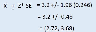
It means that we are 95% confident that college student on average have been in 2.72 to 3.68 exclusive relationship.
When do you use confidence intervals?
Confidence intervals are used to estimate the range of values that a population parameter, such as a mean or a proportion, is likely to fall within. They are used to provide a range of values that is likely to include the true value of the population parameter, based on a sample from that population.
Confidence intervals are used in inferential statistics to help draw conclusions about a population based on a sample of data. They are often used in hypothesis testing to determine whether a
difference between two groups is statistically significant or due to chance. Confidence intervals can also be used to determine the precision of an estimate, by indicating the amount of uncertainty associated with the estimate.
So, you can calculate confidence intervals for many kinds of statistical estimates, including:
- Proportions
- Population means
- Differences between population means or proportions
- Estimates of variation among groups
These are all point estimates, and don’t give any information about the variation around the number. Confidence intervals are useful for communicating the variation around a point estimate.
Calculating a confidence interval: what you need to know
To calculate a confidence interval, you need to know the following:
- The sample size: The larger the sample size, the more reliable the estimate will be, and the narrower the confidence interval.
- The sample mean: This is the average value of the
- The population standard deviation (σ) or the sample standard deviation (s): If the population standard deviation is known, it can be used to calculate the standard error of the mean. If the population standard deviation is unknown, the sample standard deviation can be used instead.
- The level of confidence: This is usually expressed as a percentage, such as 95%, and represents the probability that the true population parameter falls within the confidence interval.
- The distribution of the data: The distribution of the data should be approximately normal or the sample size should be large enough for the central limit theorem to apply.
Once you have this information, you can calculate the confidence interval using the following formula:
Confidence interval = Sample mean ± (z-score x Standard error of the mean)
where the z-score is determined based on the level of confidence and the distribution of the data, and the standard error of the mean is calculated using the sample size and the standard deviation.
Example: Calculating the confidence interval
For example, if you have a sample of 100 people and want to calculate a 95% confidence interval for the mean weight of the population, and you know the sample mean is 70 kg, the sample standard deviation is 10 kg, and the distribution of the data is approximately normal, you can use a z-score of
1.96 (based on a standard normal distribution) and the formula:
Confidence interval = 70 ± (1.96 x (10/√100)) = 70 ± 1.96 kg
This gives you a confidence interval of 68.04 kg to 71.96 kg, which means you can be 95% confident that the true population mean weight falls within this range.
Confidence interval for the mean of normally-distributed data
To calculate a confidence interval for the mean of normally-distributed data, you can use the following formula:
CI = X̄ ± zα/2 (σ/√n)
Where:
- X̄ is the sample mean
- zα/2 is the z-score that corresponds to the desired level of confidence (e.g., for 95% confidence, α = 0.05/2 = 0.025 and zα/2 = 1.96)
- σ is the population standard deviation (if known) or the sample standard deviation (if unknown)
- n is the sample size
To use this formula, you first calculate the sample mean and standard deviation. Then, you
determine the appropriate z-score for the desired level of confidence. Finally, you plug in the values and calculate the lower and upper bounds of the confidence interval.
For example, let’s say you have a sample of 50 observations from a normally-distributed population with a sample mean of 10 and a sample standard deviation of 2.5. You want to calculate a 95% confidence interval for the population mean. Using the formula above, you would get:
CI = 10 ± 1.96 (2.5/√50) = 10 ± 0.697
Therefore, the 95% confidence interval for the population mean is (9.303, 10.697). This means that we are 95% confident that the true population mean falls within this range.
Confidence interval for proportions
To calculate a confidence interval for proportions, you can use the following formula:
CI = p ± zα/2 (σ/√n)
Where:
- p is the sample proportion
- zα/2 is the z-score that corresponds to the desired level of confidence (e.g., for 95% confidence, α = 0.05/2 = 0.025 and zα/2 = 1.96)
- σ is the standard error of the proportion, which is equal to the square root of [(p * (1 – p)) / n]
- n is the sample size
To use this formula, you first calculate the sample proportion and the standard error of the proportion. Then, you determine the appropriate z-score for the desired level of confidence. Finally, you plug in the values and calculate the lower and upper bounds of the confidence interval.
For example, let’s say you have a sample of 200 people and 120 of them said they prefer coffee over tea. You want to calculate a 95% confidence interval for the proportion of people who prefer coffee. Using the formula above, you would get:
p = 120/200 = 0.6 σ = sqrt[(0.6 * (1 – 0.6)) / 200] = 0.0433 zα/2 = 1.96
CI = 0.6 ± 1.96 (0.0433) = 0.6 ± 0.0848
Therefore, the 95% confidence interval for the proportion of people who prefer coffee is (0.5152,
0.6848). This means that we are 95% confident that the true proportion of people who prefer coffee falls within this range.
Confidence interval for non-normally distributed data
When dealing with non-normally distributed data, you can use non-parametric methods to calculate a confidence interval. One such method is the bootstrapping technique.
The bootstrapping technique involves resampling the data with replacement to create multiple new datasets of the same size as the original. Then, for each new dataset, you calculate the statistic of interest (e.g., mean, median, proportion) and store the value. Finally, you calculate the lower and upper bounds of the confidence interval based on the distribution of the statistic values.
Here’s a step-by-step guide for using bootstrapping to calculate a confidence interval for non- normally distributed data:
- Collect your sample data and determine the statistic of interest (e.g., mean, median, proportion).
- Resample your data with replacement to create a large number of new datasets (e.g., 10,000). Each new dataset should have the same size as the original.
- Calculate the statistic of interest for each new
- Create a histogram or density plot of the statistic values to visualize their Use this distribution to estimate the standard error of the statistic.
- Determine the appropriate percentile values for the desired level of confidence (e.g., for 95% confidence, you would use the 2.5th and 97.5th percentiles).
- Calculate the lower and upper bounds of the confidence interval using the percentile values and the distribution of the statistic values.
For example, let’s say you have a sample of 100 observations of customer satisfaction ratings on a scale of 1 to 10. You want to calculate a 95% confidence interval for the median satisfaction rating. Using the bootstrapping technique, you would get:
- Determine the median satisfaction rating for the original sample
- Resample the data with replacement to create 10,000 new datasets of size
- Calculate the median satisfaction rating for each new
- Create a histogram or density plot of the median values and estimate the standard error (e.g., using the standard deviation of the median values).
- Determine the 5th and 97.5th percentiles of the median values.
- Calculate the lower and upper bounds of the confidence interval using the percentile values and the distribution of the median values.
For example, let’s say the median satisfaction rating for the original sample data is 7.5. After
resampling and calculating the median for 10,000 new datasets, the histogram of median values looks approximately normal with a standard deviation of 0.5. The 2.5th and 97.5th percentiles of the median values are 7.0 and 8.0, respectively.
Therefore, the 95% confidence interval for the median satisfaction rating is (7.0, 8.0). This means that we are 95% confident that the true median satisfaction rating falls within this range.


